What it is for
A Smith chart is a graphical calculator for transmission-line problems. It was invented in the 1930s to avoid complex arithmetic, and it survives because it makes the behaviour visible in a way the arithmetic does not.
Which of the following can be calculated using a Smith chart?
Impedance along transmission lines.
Which of the following is often determined using a Smith chart?
Impedance and SWR values in transmission lines.
Which of the following is a common use for a Smith chart?
Determine the length and position of an impedance matching stub.
That last one is the killer application. Finding stub length and position algebraically is tedious; on a Smith chart it is two arcs and a reading.
The coordinate system
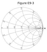
What type of coordinate system is used in a Smith chart?
Resistance circles and reactance arcs.
What are the two families of circles and arcs that make up a Smith chart?
Resistance and reactance.
What do the arcs on a Smith chart represent?
Points with constant reactance.
The features the pool asks you to name on the figure:
| Feature | Name |
|---|---|
| The large outer circle | reactance axis |
| The only straight line | the resistance axis |
| Circles tangent to the outer circle | constant resistance |
| Arcs meeting at the right-hand point | constant reactance |
| Optional third family added when matching | constant-SWR circles |
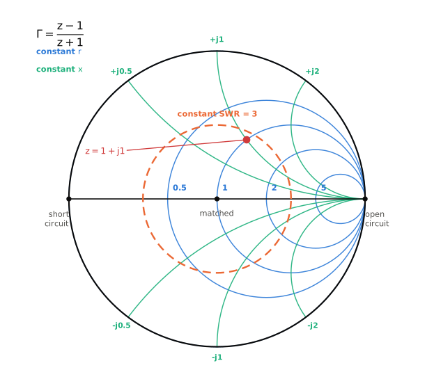
The straight horizontal line is where reactance is zero — the resistance axis — and it runs from a short circuit at the left, through the prime centre, to an open circuit at the right.
What third family of circles is often added to a Smith chart during the process of designing impedance matching networks?
Constant-SWR circles
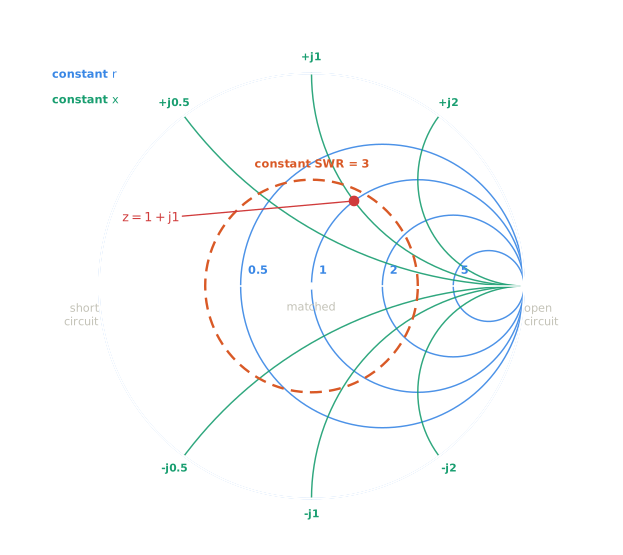
Circles centred on the prime centre. Since SWR depends only on the magnitude of the reflection coefficient, constant SWR is a constant radius — which is why moving along a lossless line traces a circle on the chart. That single geometric fact is what makes the chart work.
Why every one of those curves is a circle
The chart is a picture of one function. Normalise impedance to the system impedance, , and plot the reflection coefficient
This is a Möbius transformation — a ratio of two linear functions — and Möbius maps have a property that does all the work here: they map circles and lines to circles and lines. (A line is just a circle through the point at infinity, so it is really one rule.)
In the impedance plane, “constant resistance” and “constant reactance” are straight lines: vertical and horizontal rulings of the right half-plane. Push them through and they must come out as circles. Working out which:
\qquad \text{constant } x:\quad \left|\Gamma - \left(1 + \frac{j}{x}\right)\right| = \frac{1}{|x|}$$ Read those off. **Every constant-$r$ circle is centred on the real axis and passes through $\Gamma = +1$.** **Every constant-$x$ circle is centred on the vertical line through $\Gamma = +1$ and passes through it too.** That common point is the open circuit, which is why the whole chart appears to be drawn around its right-hand edge — every curve on it goes through that one point. Two more consequences worth having: - **$r = 0$ maps to the unit circle itself.** A purely reactive load reflects everything, so $|\Gamma| = 1$. The outer boundary is not decoration; it is the $r = 0$ member of the same family. - **The right half-plane maps to the unit disc.** Any passive load has $r \ge 0$, so it lands inside. A point *outside* the chart would mean $|\Gamma| > 1$ — more power coming back than went in — which is why a negative-resistance oscillator is drawn on an extended chart and a passive antenna never is. The plotted point is $z = 1 + j1$: $\Gamma = 0.2 + j0.4$, so $|\Gamma| = 0.447$ and SWR $= 1.447/0.553 = 2.62$. It sits just inside the SWR = 3 circle, as it must. *The circle centres and radii above are verified against scikit-rf's own mapping in `scripts/tests/test_rf_numbers.py`.* </details> ## Normalisation > **How is a Smith chart normalized?** > **Reassign the prime center's impedance value.** The chart's centre is 1.0 — a perfect match — and every impedance is expressed as a multiple of the system impedance. Set the prime centre to 50 ohms and a 100-ohm load plots at 2.0; set it to 75 and the same load plots at 1.33. Normalisation is why one printed chart serves every system impedance. ## The wavelength scales > **In what units are the wavelength scales on a Smith chart calibrated?** > **In fractions of transmission line electrical wavelength.** **Electrical** wavelength — so velocity factor is already accounted for, and the distances you read off must be converted to physical length before you cut anything. The transmission-lines lesson has the conversion. One full trip round the chart is a **half** wavelength of line, not a whole one, which follows from the half-wave repeat rule: a half wavelength returns you to where you started. ## Why it is worth learning despite the calculators A NanoVNA draws a Smith chart on its screen, so the chart has outlived the arithmetic it replaced. What it gives you is **intuition**: - Moving along a line is rotation. Clockwise toward the generator. - A high-SWR load is far from centre; matching means moving inward. - A series reactance moves you along a constant-resistance circle; a shunt reactance moves you along a constant-conductance circle. That is the whole design procedure for an L-network. None of those are visible in a table of numbers. ## Check yourself 1. What does the only straight line on a Smith chart represent? 2. A load plots at 2.0 + j0 on a chart normalised to 50 ohms. What is the actual impedance, and the SWR? 3. How much line does one complete rotation around the chart correspond to? <details> <summary>Answers</summary> 1. **The resistance axis** — where reactance is zero. 2. 2.0 × 50 = **100 ohms resistive**, and SWR = 100/50 = **2:1**. 3. **A half wavelength** of electrical length. </details>